Formula
A Nectari Formula is an Excel-like formula called NecAccess that, when called, can retrieve enterprise data from your databases.
Nectari Formulas can be manually created or they can be easily generated using the Nectari Formula Editor dialog window provided with the Add-in.
To create a new Nectari Formula using the Nectari Formula Editor, do the following:
- Click on
 Formula Wizard in the Excel Add-in tab to open the Nectari Formula
Editor.
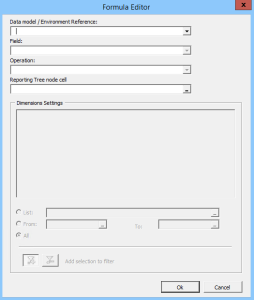
- Select the Reference corresponding to the Data Model and the Environment you want to use to access the data you need.
- Select the Field corresponding to the data to display with this formula.
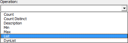
- Select the Operation. There are many operations available:
- Count:
- To return the number of values for the selected field.
- Count Distinct:
- To return the number of distinct values for the selected field.
- Description:
- To specify that the selected field should actually return description type data.
- Min:
- To return the minimum value for the selected field.
- Max:
- To return the maximum value for the selected field.
- SUM:
- To return the sum value for the selected field.
- SUM (Reversal):
- To return the sum reversed for the selected value, could be used as an example for the sales revenue inside an income statement.
- SUM (Debit):
- To return the sum value only if the total of the sum is a debit for the selected value.
- SUM (Credit):
- To return the sum value only if the total of the sum is a credit for the selected value.
- List:
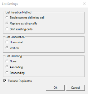
- To retrieve the list of values for the selected field. There are a few ways to display the
list in Excel according to the choices made for list insertion method, list orientation
and list ordering properties in the Setup window. This window shows up when the List
option is selected as operation (see figure below).
- Single Comma Delimited Cell:
- This is used to place the values into the current cell in a comma-delimited format.
- Replace Existing Cells:
- This is used to place the first value in the current cell and place the following values in adjacent cells while overwriting the content of those cells.
- Shift Existing Cells:
- This is used to place the first value in the current cell and the following values in the adjacent cells while shifting the content of those cells.
- Horizontal
- : To use the horizontal adjacent cells when placing the list values in many cells.
- Vertical:
- To use the vertical adjacent cells when placing the list values in many cells.
- None:
- No specific sorting order.
- Ascending:
- To sort the list in the ascending order.
- Descending:
- To sort the list in the descending order.
- DynList:
- To return the list of values for the selected field. The output is a comma delimited cell sorted in ascending order. The difference with the other list option is that this list will update as any Excel formula when the parameters are changed.
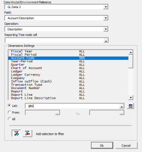
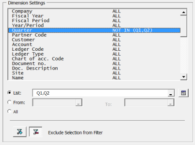
- Specify the Dimension Settings by selecting the Dimension from the list of dimensions so that it gets highlighted then choosing one of the three filtering options available under the list area.
This section is used to filter the records used within the calculations for the selected field and operation. You can enter those filtering settings for as many Dimensions as you like.
- In the Reporting Tree node cell field, select the reference cell you defined in Reporting Tree.
When you change the Reporting Tree node cell field, the formulas will automatically be refreshed.
- List:
- To specify a list of values that should be included or excluded for the selected Dimension.
- To determine if the values should be included or excluded, use the buttons Add
Selection to Filter and Exclude Selection from Filter that show up when the
List option is selected .

- You can specify a unique value or a list of many values.
- You can manually enter values separated by a comma.
- For example, you can
decide to exclude Quarters Q1 and Q2 by entering Q1, Q2 in the List field
and by selecting the Exclude selection From filter button.
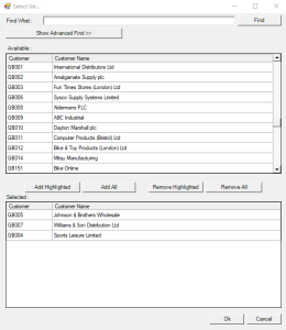
- You can use the
 Prompt button next to the List field to select a range
of values from the Prompt associated with the Dimension. In the Select List
window that appears, you can select the values you want to include (or exclude)
from the Available list (up) and use the Add Highlighted button to add them
to the selected list (below). You can also Add All, Remove All or remove some
values from the Selected List area (Remove Highlighted).
- Using the
 Lookup button of the List field, you can get the value from an
Excel cell, which can contain either one value, or multiple values separated by
the default list separator.
 - From .. To:
- To specify a range of consecutive values to include to (or exclude from) the filter for the Dimension, the first one being entered or selected in the From: field, and the second one in the To: field. The way to enter values in each of those two fields is the same as for the List: field, as presented above.
- All:
- Not to apply any filter for the selected Dimension. This is the default value.
The resulting Nectari formula can be seen in the Excel formula bar.
Here, we display the Account Description for the Account Code contained in the $B6 cell. See the setup for the formula below.
The Nectari Add-in for Excel was developed to enable Nectari Formulas to work in the same manner as any other Excel function.
In other words, Nectari Formulas can be copied, pasted, and dragged from cell to cell. Performing these operations on a formula containing absolute or relative cell addresses will automatically adjust as required to the same extent that they would within a Sum function. Exceptions to this rule are formulas using the List operation.
This type of operation which can affect cells adjacent to the active cell should not be automatically refreshed when recalculating a worksheet to avoid accidentally overwriting cells. As such, this type of formula is not saved into the cell as a regular Excel formula. It is saved into the cell as an Excel Cell Comment, which does not automatically get processed when refreshing the worksheet and is not an adjust cell when copied between worksheet cells.

