Cache Optimizer
The cache optimizer feature was designed to provide users with recommendations on how to enhance the performance of their Excel Add-in reports and minimize workbook refresh times. It accomplishes that by analyzing the user's references and generated Nectari formulas to produce a report that outlines how they can be improved.
The cache optimizer works in two parts:
- It performs a detailed analysis of an Excel workbook's formulas and content.
- It provides recommendations on how to optimize the workbook's references and formulas. Users can then easily implement those recommendations via the cache optimizer, if they so choose.
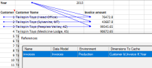
Here you have a basic report that displays the invoice amount for every customer from 2013.
The invoice amount is a Nectari formula that filters based on both year and customer ID. In this example, the reference configuration has been set to cache based on the year, customer ID and invoice number.
By using the cache optimizer feature, the following results can be obtained:
It is recommending that the user remove the year field from their reference configuration. To do so, they would simply click the Apply changes and recalculate button.
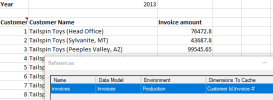
The result is shown in the image below:
As you can see, the year field has been removed from the reference as per the cache optimizer recommendation, and all of the data has been recalculated.
The cache optimizer feature provides recommendations intended to improve formulas but it is important to understand that its recommendations may not always be ideal for your specific report.
For example, imagine that you receive a cache optimizer recommendation to remove the year field from the cache as all formulas filter on the same year at the time of the analysis. But then, later on, multiple year values are added making it preferable to cache the year field. For reasons such as that, it is important to view the cache optimizer recommendations as useful hints rather than absolute truths.
Performing an Analysis
Before using the cache optimizer, ensure that you are connected to your central point and that you have the workbook that you wish to analyze open.
To perform an analysis using the cache optimizer feature:
- In the Excel Add-in ribbon tab, locate and click the
button.
-
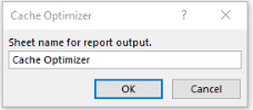
Enter a sheet name for your optimization report in the pop-up window and then click OK. Please note that you cannot use the name of an existing sheet.
-
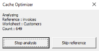
The cache optimizer will begin its analysis and you will be able to track its progress from the pop-up window.
-
Stop analysis - Stops the analysis at its current stage of progress. Clicking this button will generate a report containing only the references that were already completely analyzed. If no references were completely analyzed when the button was selected, no report will be generated.
-
Skip reference - Skips the reference that is currently being analyzed and omits it from the final report. No report will be generated if all references are skipped.
-
The duration of the analysis can vary considerably depending on the size of your workbook.
-
Once the analysis is complete, a new sheet containing the output is automatically generated and added to the workbook.
The cache optimizer will only produce a recommendation output if your currently active workbook contains Excel Add-in references and formulas.
Applying Recommendations
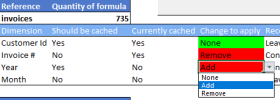
Once the optimization report is complete, you can choose to either accept and apply the advice to your workbook or not. If you wish to apply the recommendation, you can input the changes manually from the reference configurator or automatically by following the steps below:
- Review all of the recommended changes. Possible recommendations are:
- To remove a dimension from your references (highlighted in red).
- To add a dimension to your references (highlighted in red).
- To leave the dimension unchanged (highlighted in green).
-
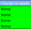
You can customize the recommendations before applying them by clicking the cell in the Change to apply column and selecting a behaviour from the drop-down list that appears.
- Once all of the dimension changes are customized to your liking, click the
button at the top of the optimization report to apply the changes.
The Apply changes and recalculate button will only work if you are currently using the same UI language as you were when the optimization report was generated.
