Pivots

Worksheets with Pivot Tables (i.e Cross-Tab Worksheets ) displays the data in a different view.

It allows specific sets of data to be summarized and analyzed by spreading values from specific Fields into columns. The Pivot Layout is very useful for comparing numeric data for different occurrences of one or several Fields called Pivot Fields.

In order to create a Pivot Layout:

1. Start from an ordinary worksheet.
2. Select the Field you want to assign as the Pivot then drag and drop that Field to the chosen location.
   Example

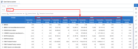
   Here we chose the Open Order by Customer view which contains order history by Product Category. A cross-tab worksheet allows the user to compare sales for different years. Each year is displayed as a column set and would contain three columns: Dollars, Quantity and Margin. In this case, the Pivot Field is the Year.
   

   The final result looks like this:
   

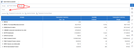
   Note

   It is possible to include more than one Field in the Pivot section.

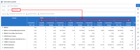
In the previous example, if the field Month is added, each value of the field Year is combined with distinct values by Month.

As a result, the top header appears as the Year:

To display a Grand Total for a particular pivoted column:

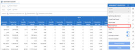
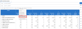
• In the Columns section, right-click on a Measure and select Show in Pivot Total.
  
  Note

  This will display a new column at the far right of the screen by default.

• Apply Show in Pivot Total to multiple Measures (Columns) if desired.

The Total Column can be displayed at the beginning or at the end of the Pivot section. To change the position:

1. In the Settings menu (right panel), click on .
2. Under the General section, drag the Show Total Front slider to the right to turn it on. The columns will change automatically.