Nectari Pivot Table
The Nectari Pivot Table feature is a powerful way for you to easily pull out data in the form of a Cube without extracting the raw data to Excel first. Only use Nectari Data Models to get the required data.
To create a Nectari Pivot Table, do the following:
- Click on
Pivot Table in the Excel Add-in tab.
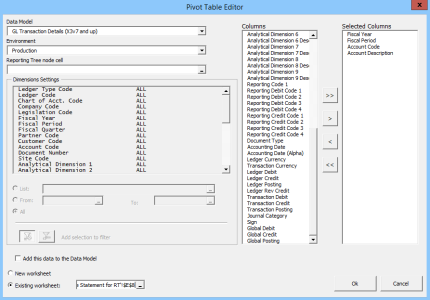
- In the Nectari Pivot Table Editor window that appears, choose the Nectari Data Model, the Environment and enter the Dimension Settings to filter the resulting data (the same way as for a Nectari Formula, refer to Formula for more details).
- Select the columns to be used with the > and < arrows.

If you set up a cell for the Reporting Tree Node (refer to Reporting Tree), the Pivot Table feature will automatically use the Reporting Tree as a filter.
Please note that changing the Node in the Reference Cell (the one containing the Reporting Tree Node) will not trigger automatically the Pivot Table Refresh feature. You have to click on Pivot Table Refresh to update the table based on your new selection of the Reporting Tree Node.
- At the bottom of the Nectari Pivot Table Editor window, choose if you want the result to be displayed in a New Worksheet, or in the same worksheet (Existing Worksheet). In the case you select existing worksheet, you need to specify the starting cell in the field.
- Click on OK to let the resulting Cube be made available in the workbook.
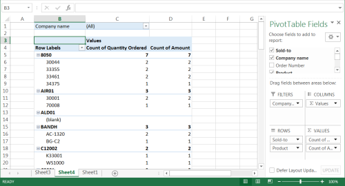
- You can then use it
as a regular Excel Pivot Table by adding Values, Filters, Rows and Columns to the Report area.

Pivot Table Refresh
The Pivot Table Refresh feature is used to refresh the Pivot Table results with up-to-date data from the database.