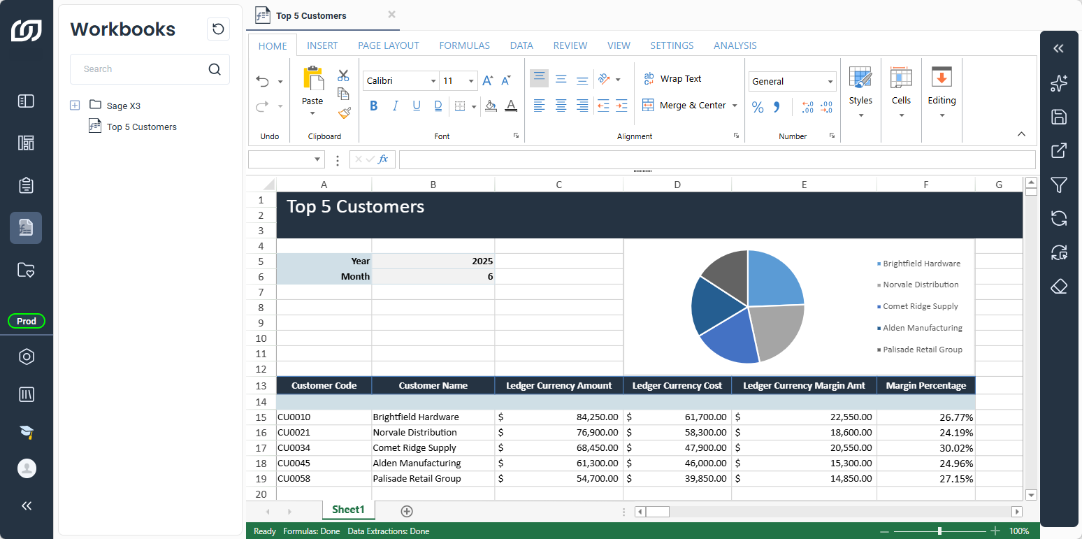
Example: Top 5 Customers by Sales

This example builds a data extraction from scratch, covering the workbook setup, the extraction table, the filters, and a margin percentage calculation. The finished table ranks the top 5 customers by sales for a selected year and month, along with their margin percentage, and the pie chart updates automatically whenever the filter values change.

important

To follow along, the Invoice Analysis data model needs to be installed and accessible in the environment.

01

Prepare the workbook

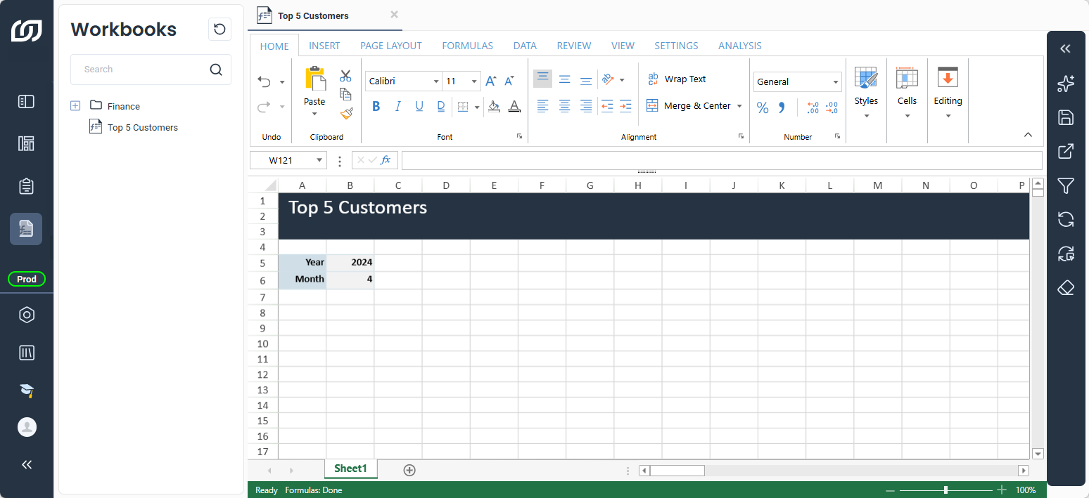
Two cells hold the year and month, to be referenced as filters later. Once referenced, changing either cell updates the results automatically.

1. Select Classeurs in the navigation panel.
2. Right click and select New Workbook.
3. Name the workbook Top 5 Customers and click Save.
4. In cell A5, enter Year, and in cell B5, enter 2024.
5. In cell A6, enter Month, and in cell B6, enter 4.
6. (Optional) Apply any formatting, such as a title or fill colors.

02

Create the extraction table

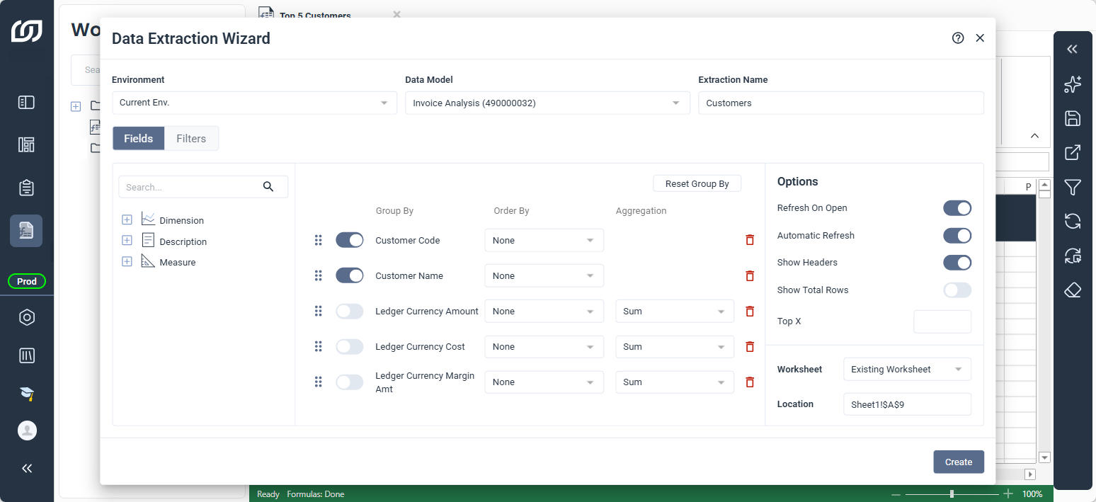
The extraction identifies each customer and totals their transactions, grouped by Customer Code and Customer Name with the three ledger fields summed.

1. Select cell A9.
2. Select the Analysis tab, then click Data Extraction Wizard.
3. In Environment, select Current Environment.
4. In Data Model, select Invoice Analyses.
5. Name the extraction Customers.
6. In the Fields tab, search and add the following fields:
   • Customer Code
   • Customer Name
   • Ledger Currency Amount
   • Ledger Currency Cost
   • Ledger Currency Margin Amt
7. Under Order By, leave every field as None.
8. Under Aggregation, untoggle the three ledger fields and set them to Sum.
9. Click Create.
10. (Optional) Apply any formatting.

03

Add filters

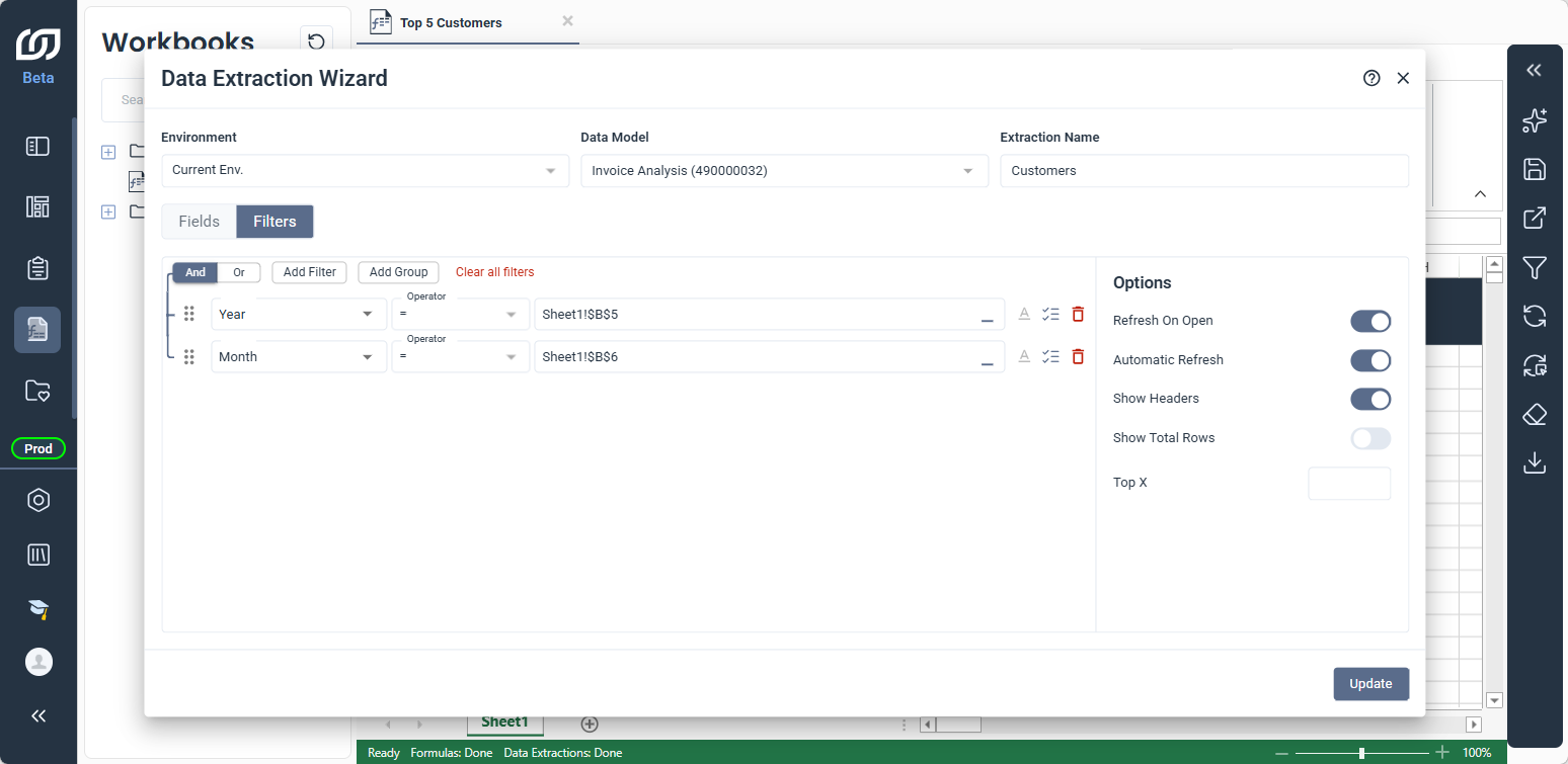
Adding filters connects the extraction to the Year and Month cells. Once connected, changing either cell updates the extraction results automatically.

1. Select any cell in the extraction table.
2. In the Analysis tab, click Data Extraction Wizard.
3. Click the Filters tab, then Add Filter.
4. In the first dropdown, search for the Year field.
5. Keep the operator as = and click cell B5 directly in the sheet.
6. Click Add filter to add another one.
7. Search for the Month field and click cell B6.
8. Click Update.

04

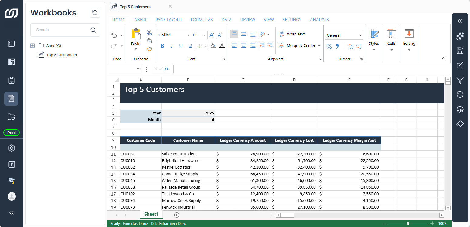
Filter to June 2025

Filtering to June 2025 narrows the extraction to that month's transactions, showing which customers ranked highest during that period.

1. In cell B5, change the year to 2025.
2. In cell B6, change the month to 6.
3. The table refreshes automatically with the updated results.

05

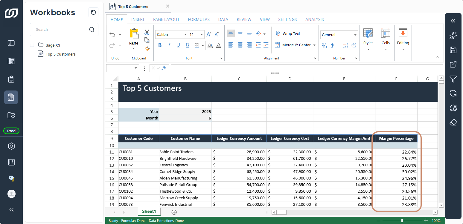
Add a margin percentage column

The formula divides the margin amount by the ledger amount for each customer, turning the two raw totals into a single percentage that shows how profitable each customer is.

1. Right click the last column header cell E9.
2. Hover over Insert and click Table Columns to the Right.
3. Rename the new column header to Margin Percentage.
4. In the first row of the new column, enter =E10/C10.
5. Select the whole F column.
6. In the Home tab, select Percentage from the Number dropdown.

06

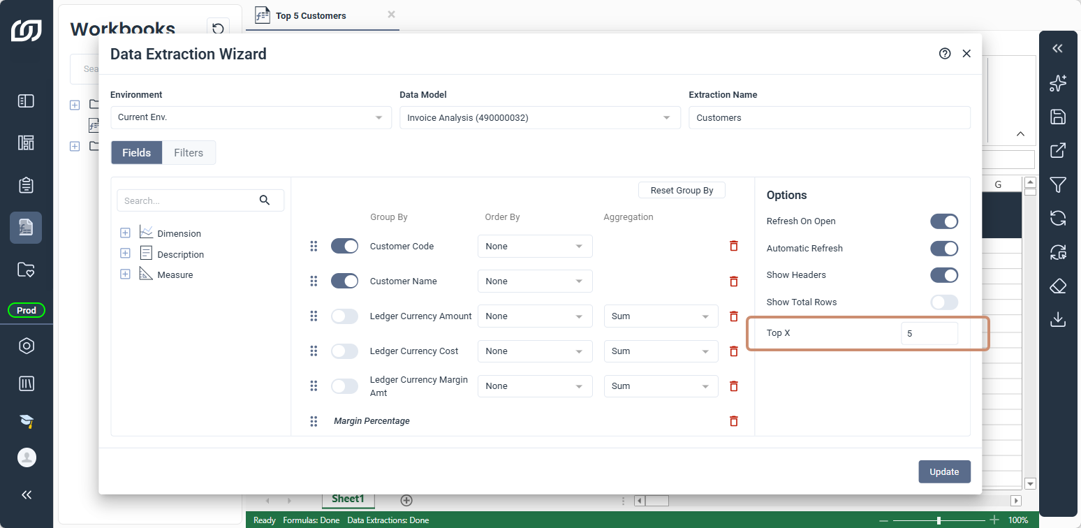
Limit to top 5 customers

Setting a Top X value narrows the table to the highest ranked customers by ledger currency amount.

1. Select any cell in the extraction table.
2. In the Analysis tab, click Data Extraction Wizard.
3. Under Options, set Top X to 5.
4. Click Update.

07

Build a pie chart

The chart is linked to the extraction data. Changing the year or month filter values updates both the table and the chart automatically.

1. Select the Customer Name and Ledger Currency Amount columns.
2. Select the Insert tab, and click Charts.
3. Under Pie, select the pie chart, then click Ok.
4. (Optional) Click the new chart, and in the Chart Design tab, apply any formatting.
5. Move the chart on the sheet as needed.